
Excel: Structured References and Data Validation

Preamble
I am going to show you how to use data validation rules based on Excel table structured references. At the end of this article, I’ll attach an Excel workbook for you to study.
Scenario
Let’s say we want to create an Excel table to game out possible flight trips with multiple legs. We might want to include departure and arrival times for each respective leg.
Let’s also say we want to assert a rule: arrival date-times must come after departure date-times. How might we solve this problem in a robust manner?
Approaches
Indication
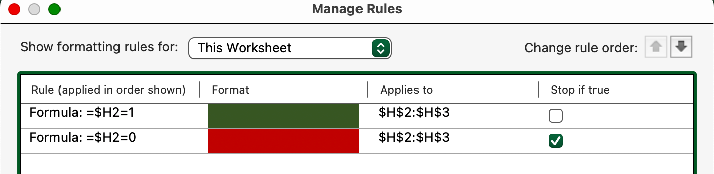
As an aside, consider that indicating a logical relationship between cells (EG: with conditional formatting) is distinct from enforcing a logical relationship between cells (EG: with data validation).
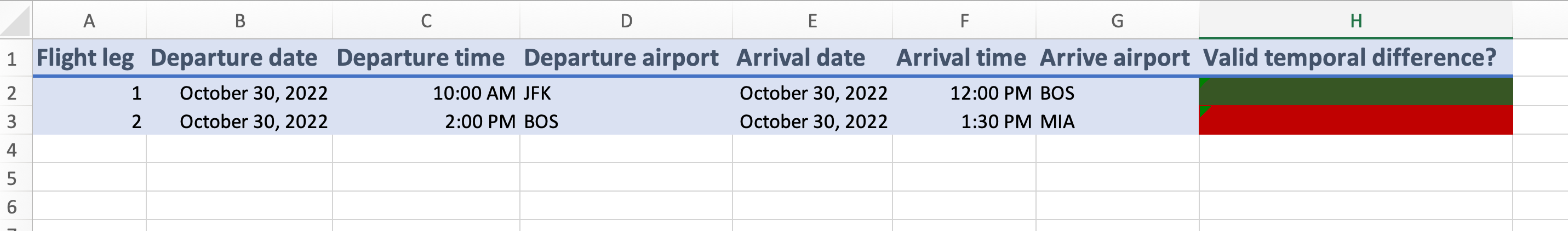
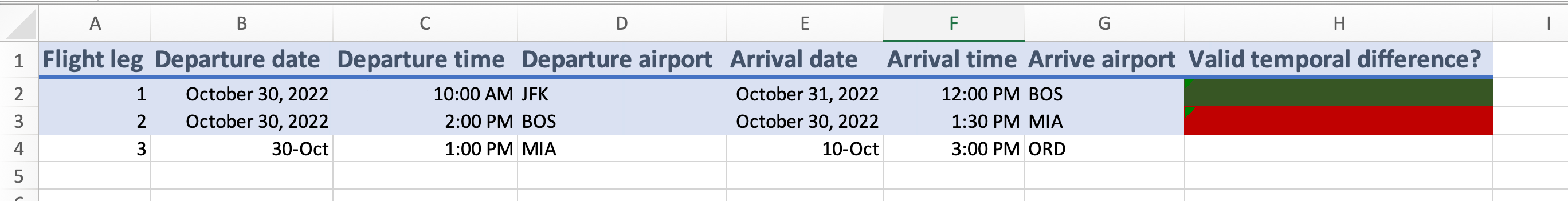
In this first approach, we set some crude conditional formatting rules to indicate an arrival time that’s earlier than a departure time for any given row.
In the second row, we can see that I’ve made an error by entering an arrival time (1:30 PM) that’s earlier than the departure time (2:00 PM).
By using conditional formatting, we can indicate a mistake (with the color red, in this case).
Data Validation with Standard Cell References
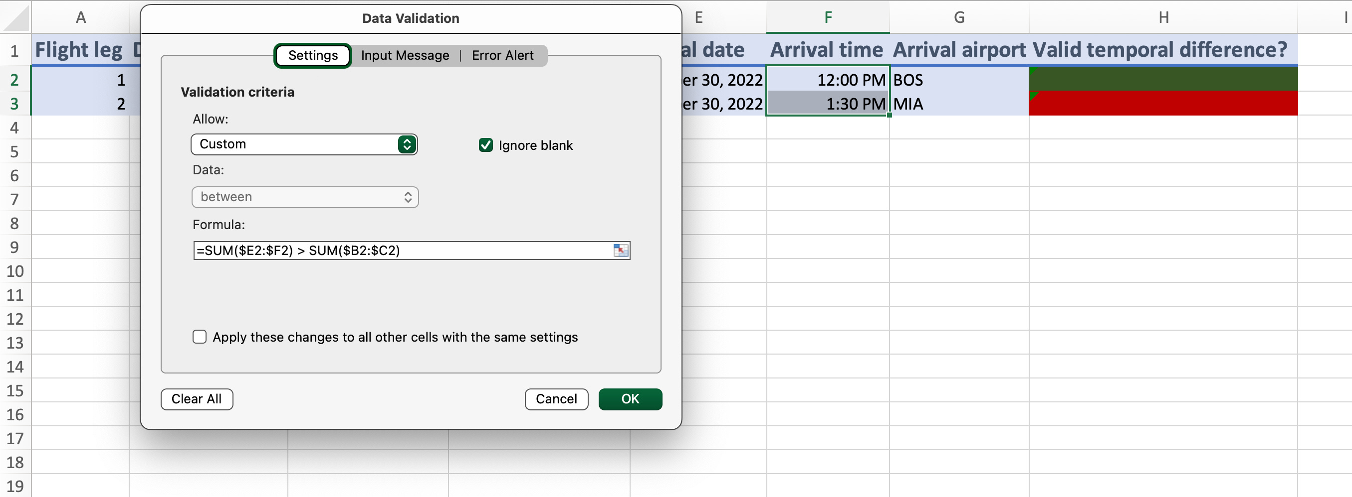
Let’s start by recalling the rule we want to enforce: the arrival date-time should be ahead of the departure date-time.
With this approach, we compare the sum of the Arrival date and Arrival time columns to the sum of the Departure date and Departure time columns.
# Example 1 data validation formula
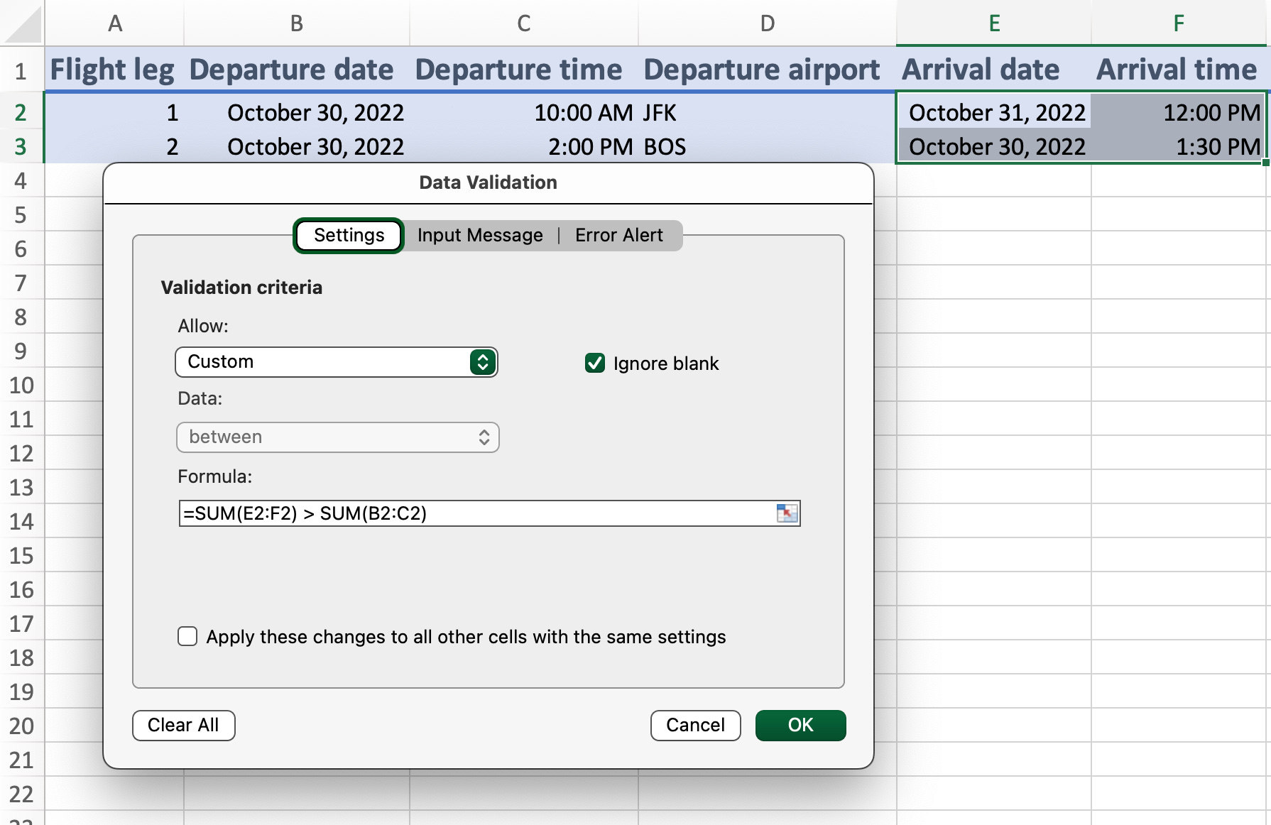
=SUM(E2:F2) > SUM(B2:C2)So, this seems to work at first; but, not really.
Problem 1
Despite setting the data validation rule `SUM(E2:F2) > SUM(B2:C2)` for the range E2:F3, the effective rule for column F is wrong: instead, the rule attempts to sum column F (Arrival time) and column G (Arrival airport).
Problem 2
If we try to add a third row, our rules and formatting aren’t automatically applied.
Before going on to a structured references example, I should add that it is perfectly possible to make our table work with standard cell references. The trick is to use “mixed” cell references. In this case, “mixed” means using a reference with both a column-absolute reference and a row-relative reference.
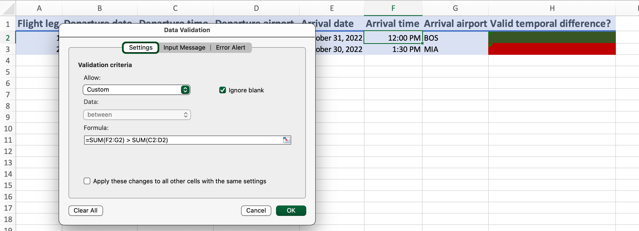
# Our data validation rule using mixed references.
=SUM($E2:$F2) > SUM($B2:$C2)
After making the above tweak to the rule we applied to the range E2:F3, we can see that column F has a data validation rule with the desired cell references.
What about adding more rows? To carry over the data validation and formatting rules, the quickest way is to select the entire empty row below our data (IE row 4) and use Excel’s functionality for duplicating the states of the above row.
The downside of this approach is that we wind up with the data of row 3 as well; of course, we could clear the cell values.
So, it is perfectly possible to use manually managed tables by carefully duplicating the various kinds of rules we want when adding additional data.
However, there is a better way: use Excel tables and structured references.
Data Validation with Structured References
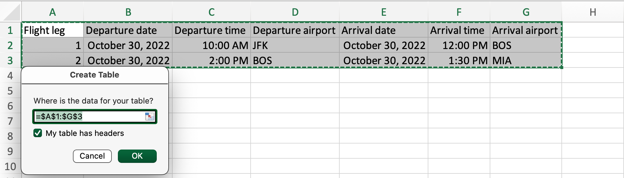
To save a bit of time, I’ve used paste-special to copy over the values and number formatting rules from our manual table to another spreadsheet.

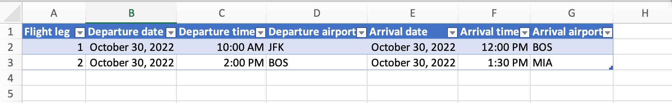
We next convert the range A1:G3 into an Excel table.
Quick review of (most) kinds of structured references:
# The name of our table is Table1, which was automatically assigned by Excel and always refers to the present range of the Excel tab.

# A reference to the entire table, including the header row.
=Table1[#All]

# A reference to just the data portion of Table1
=Table1

# A reference to just the header row of Table1
=Table1[#Headers]

# A relative reference to the Arrival date column, data only
=Table1[Arrival date]

# A relative reference to the Arrival date column, data and header
=Table1[[#All],[Arrival date]]

# An absolute reference to the Arrival date column, data only
=Table1[[Arrival date]:[Arrival date]]

# An absolute reference to the Arrival date column, data and header
=Table1[[#All],[Arrival date]:[Arrival date]]

# A relative reference to "this" row and the Arrival date column
=Table1[@[Arrival date]]

# An absolute reference to "this" row and the Arrival date column
=Table1[@[Arrival date]:[Arrival date]]
We’re not interested in the Arrival date column only, as we want to reference the sum of the Arrival date and Arrival time columns on a row by row basis in order to properly compare arrival and departure times.
# A relative reference to "this" row and the Arrival date and Arrival time columns. Note that this reference is column-absolute.

=Table1[@[Arrival date]:[Arrival time]]
It looks like the data validation rule we want to apply is this:
=SUM(Table1[@[Arrival date]:[Arrival time]]) > SUM(Table1[@[Departure date]:[Departure time]])
Let’s give it a go.
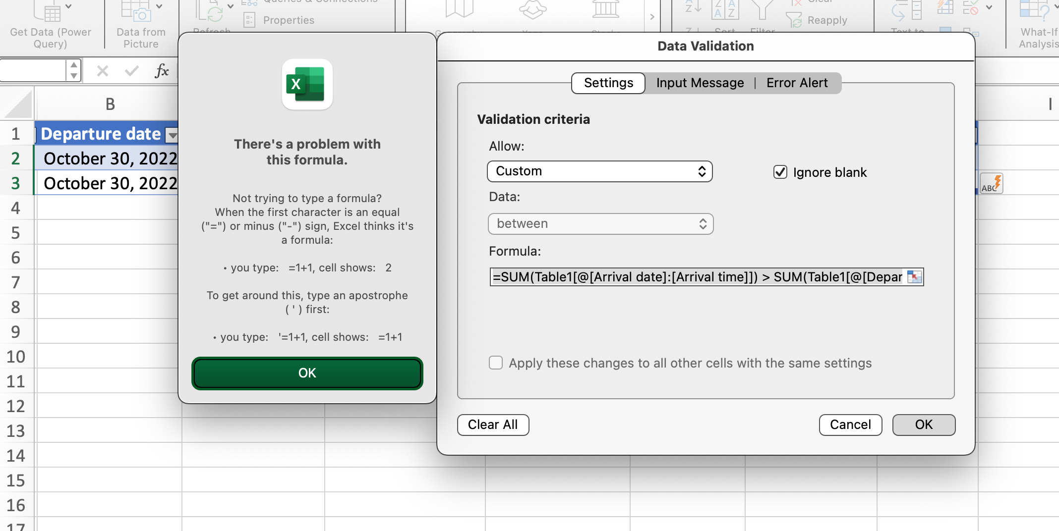
Uh oh! This doesn’t work. For some reason, we can’t use structured references in data validation rules.
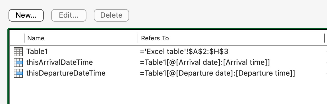
Don’t worry; there is a solution. Enter “named ranges” — another kind of range reference that we can use in data validation rules.
Using our knowledge of structured references, we’ll define the named ranges “thisArrivalDateTime” and “thisDepartureDateTime”. In this context, “this” merely denotes that we’re referencing the row in which a rule is applied. EG: `=Table1[@[Arrival date]]`.
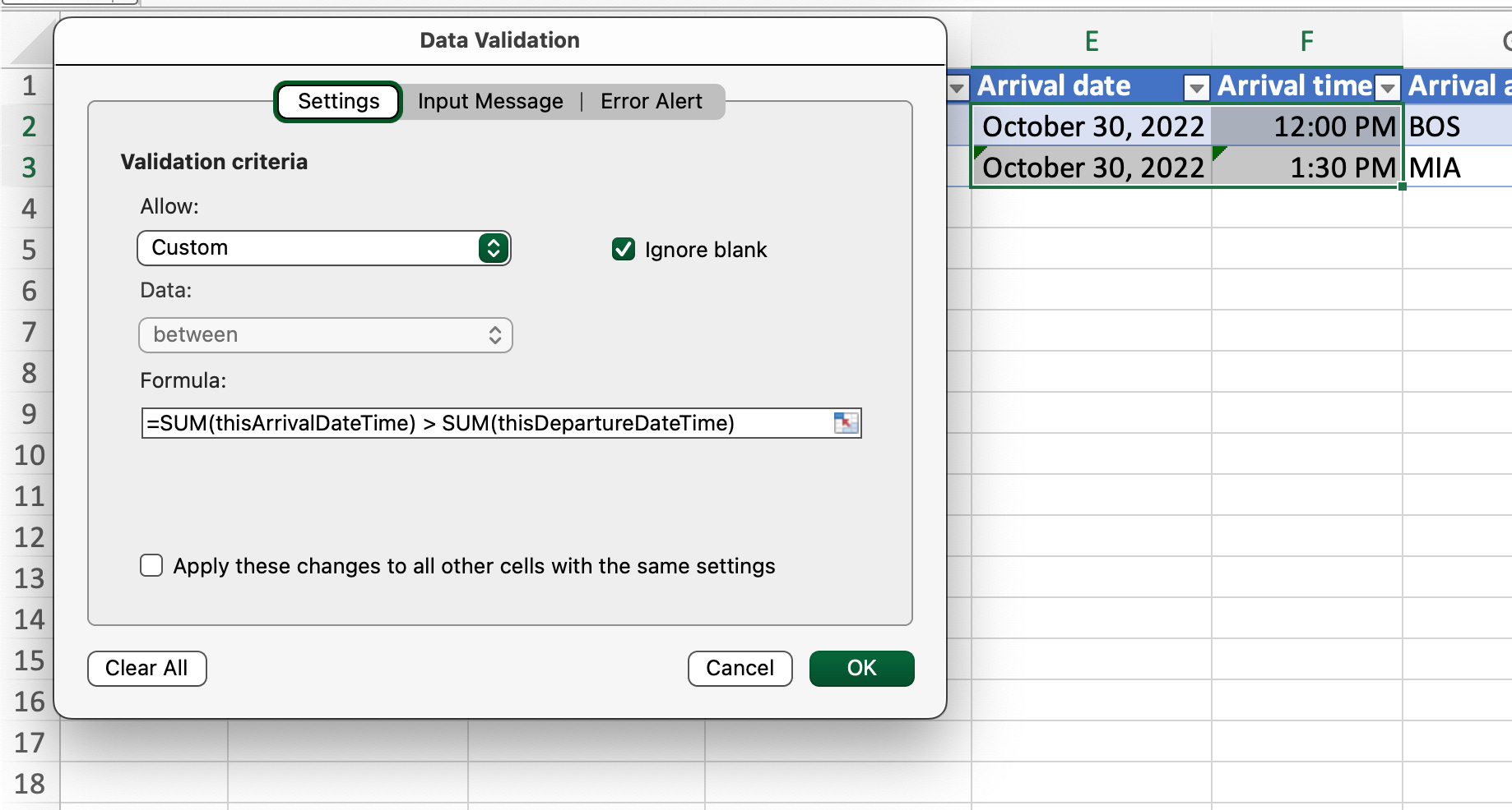
Using the above named ranges, our data validation rule for the Arrival date and Arrival time columns looks like this.
Let’s test this out by setting Arrival date and Departure date as “October 30, 2022”, but attempt to set the Arrival time before the Departure time.
As expected (and hoped), our rule successful prevented setting an Arrival time before the Departure time.
Now, let’s try clearing the Arrival date and Arrival time columns; then, let’s try setting an Arrival date earlier than the Departure date.
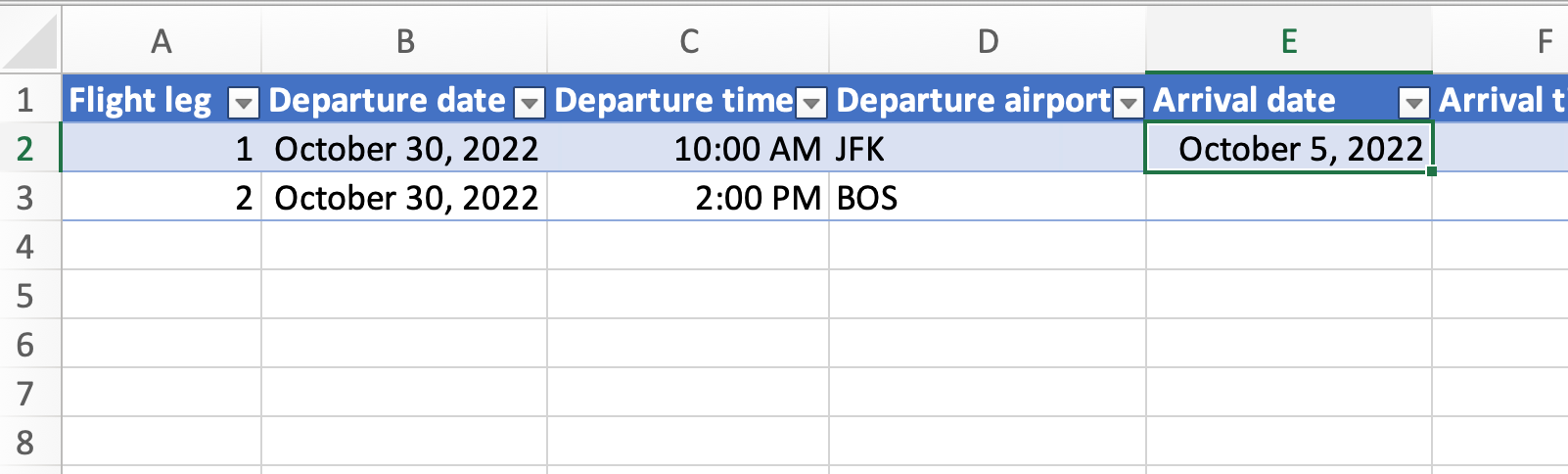
Oh no, why were we allowed to enter an Arrival date earlier than the Departure date?
Our mistake was leaving the data validation option “ignore blanks” enabled.

I can’t say I know why this messes things up for us, but I can say that unchecking this option allows our data validation rule to work as expected.
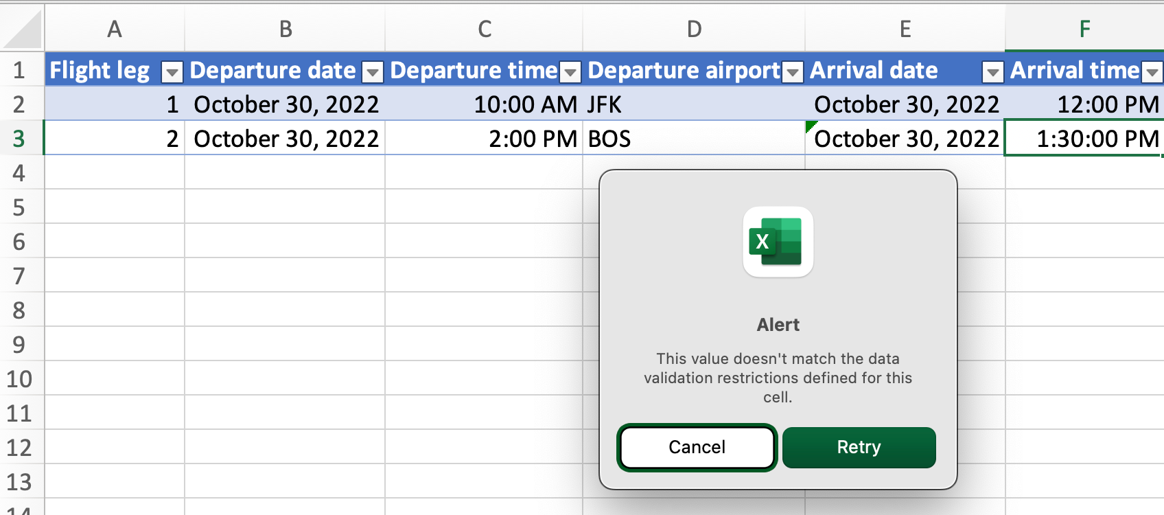
Now, with Arrival time empty, we try to set an Arrival date before the Departure date.
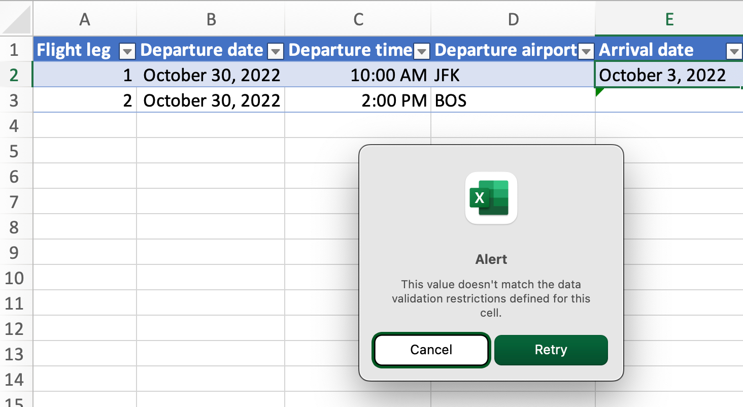
Our validation rule successfully catches the error!
Note, that trying to add an Arrival time while Arrival date is blank will also fail. This is because the `SUM()` function treats an empty cell as a 0. Zero, in Excel, is typically equivalent to the unreal date-time “January 0, 1900 12:00 AM”.
Summary
We started off with a goal of tracking the legs of a flight trip in an Excel spreadsheet, and we also wanted to prevent the inclusion of an arrival date-time that was equal or less to a departure date-time.
We demonstrated that conditional formatting could be used to indicate such a mistake.
We demonstrated that standard cell references could be used for data validation successfully as long as we were careful to avoid certain pitfalls.
We demonstrated that our goal could be achieved robustly with the combination of an Excel table, named ranges, and structured references.
Lastly, I’ve attached a copy of the Excel workbook I used for writing this article. Have fun.
Outro
If you enjoyed this entry, consider becoming a subscriber. As a subscriber, you’ll be able to comment on all my articles.
Please feel comfortable sharing honest critique.
Thank you for reading.